Speaker Simulation

This short article follows an example in the Book 'Elektroakustik' by Zollner, M., & Zwicker, E. (2013). It is not quite suitable for beginners in these matters, still it represents a simplified model of an electroacoustic system: A dynamic speaker. It tries to model the speaker's internal electrical components, its membrane and the interaction with air. Essentially, the question is answered how 'loud' a sound will be in 10 meters distance, given an input voltage to the speaker.

Since the book itself is written in german, some of the german terminology is kept in order to make this accessible/less confusing for german native speakers.

The example we go through here is 'Example 6.2'. It's text reads as follows:

"A dynamic bass speaker is placed in an infinite wall. What is the observed active sound power (Wirkleistung $P_L$)? What is the observed Sound Pressure Level ($L$ in dB) in 10m distance, disregarding/including theoretic index of directivity?"

These are the given parameters:

• voltage source, the input voltage, $U_i$, 3 V.
• Internal resistance of the voltage source $R_o \approx 0 \Omega$.
• Radius of the membrane, $a=12cm$.
• Mass of the membrane, $m_M=40g$.
• Stiffness of the membrane(-mount), $S_M=7000N/m$.
• Mechanical resistance of the membrane(-mount), $W_M=3Ns/m$.
• Resistance of the speaker coil, $R_s=6\Omega$.
• Inductivity of the speaker coil, $L_s=0.5mH$.
• Transducer coefficient $\alpha=10N/A$.

Solution

There are 2 major things to unpack here:

• The interaction of the electric/mechanic/acoustic systems and their modelling.
• An infinite wall around the speaker and its effects.

Piston Membrane in an infinite Wall

For mathematical simplification, a so called piston membrane ('Kolbenmembran') is assumed. This means that all points on the membrane have the same velocity. It sits in an infinite wall for mathematical simplification as well.

Basically, the little portion of air that sits in front of our membrane creates a load with certain properties. These properties can be modelled by a mechanical mass and a mechanical resistance (a force that is dependent only on velocity). This is what is meant from hereon when we say slightly weird things like 'the mass of air'.

Before going deeper on the acoustic side of things below, we model the system making use of 2 simplified values we get from this assumption:

• The mass of air shall be $m_L = \frac{8}{3} \varrho a^{3}$.
• The resistivity of air shall be $W_L = 4.5 Z_0 a^2$.

Here $\varrho$ is the density of air and $Z_0$ is the characteristic acoustic impedance of air.

Having said that, we will turn to a diagram of a 'normal' simplified speaker and identify the elements that will be modeled.

Modeling using Electrical Equivalent Circuits

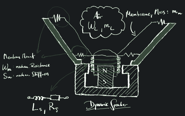
Looking at the above Figure it is obvious we have three different domains:

• electric
• mechanic
• acoustic

Luckily, all of this can be modelled using electrical analogons to the mechanical domain. This little article cannot explain all of this, but there are resources on the web and in the book explaining this in greater detail (See references Section at the end of this article). For now, its sufficient to say that here we will draw an analogy (the 'Force/current analogy', 'FI-Analogy', 'mechanical analogue I') between:

• Force and current
• Velocity and voltage
• mass and capacity
• mechanical stiffness and electrical inductivity
• mechanical resistance and electrical resistance

This gives us the ability to model almost the whole behavior of the system with one electrical circuit (This ignores any non-linearities and has other caveats).

The book gives us methods to estimate the answer using various very valuable approximations, which not only offer simplified mathematical tools but also easier insight into the behavior of the systems. Here, this will be outlined shortly, but mainly we will use th powerful lcapy python package.

So let's draw the circuit using a netlist:

from lcapy import Circuit
cct = Circuit(r"""
P1 1 0; down,  v=U_{in}
LS 1 2 {L_S}; right
RS 2 3 {R_S}; right
W 3 4; right
mM 4 10; down
rM 5 11; down
kM 6 12; down
W 0 10; right
W 10 11; right
W 11 12; right

W 4 5; right
W 5 6; right

W 6 7; right
mL 7 8; right
rL 8 13; down
W 12 13; right

W 8 9; right
W 13 14; right

P2 9 14; down, v={v_{out}}
;;\node[gray,draw,dashed,inner sep=3mm,anchor=north, fit=(1) (3) (0), label=Electrical] {};
;;\node[gray,draw,dashed,inner sep=3mm,anchor=north, fit=(4) (6) (10) (12), label=Membrane] {};
;;\node[gray,draw,dashed,inner sep=3mm,anchor=north, fit=(7) (8) (13), label=Air] {};
; color=gray, draw_nodes=connections, label_nodes=False, label_ids=False
""")
cct.draw(scale=0.5, style='european')

There are many things to be said here:

• lcapy calls springs $k$ (this is very common in the literature, see Hooke's Law) and mechanical resistances $r$. We have settled for $S$ and $W$, sticking to the book's taxonomy.
• lcapy in general is able to simulate a mixture of mechanical and electrical components. Since it recently switched its internal analogon from II to I, we will for now do this conversion ourselves. Also, this allows us to configure the transducer coefficient $\alpha$.
• Typically, this circuit should include the transducer (converting from electrical to mechanical).
• The output port of the circuit is labeled $v_{out}$, since voltage is analogues to velocity. We will create the electrical model and measure voltage, and use it to calculate power.
• The decision has been made to draw this circuit in European style but from now on we will switch to American style. The reason for this is that in American style, a spring looks very similar to a resistor and the inductor is also not far off visually.

Next, let's import modules and let python know about all our variables and constants.

from lcapy import R, C, L, f
import numpy as np
import matplotlib.pyplot as plt
import sympy
plt.style.use('website')
π = np.pi

# -- Variables given from the Text --
a = 12*1e-2 #m, membrane radius.
m_M = 40*1e-3 #kg, membrane mass.
S_M = 7000 #N/m, membrane stiffness
W_M = 3 #Ns/m, mechanical resistance, membrane 
R_S = 6 # Ω internal coil resistance.
L_S = 0.5*1e-3 #H inductivity of the coil.
α = 10 #N/A, transducer coefficient.

U_i = 3#V, input voltage
R_i = 1e-8 #Ω, voltage source, internal resistance (approx 0Ω)
dist = 10 #m, distance to speaker.

# -- Definition of physical 'constants'
ϱ = 1.2 #kg/m³, Density of air approx
I_0 = 10**-12 #W/m^2, Reference-Sound intensity (Schallintensitaet)
c_L = 343 #m/s, Speed of Sound in Air (approx)
Z_0 = ϱ*c_L # ~414. #Ns/m³, characteristic acoustic impedance (Schallkennimpedanz) of air at 20⁰C

Now, let's calculate the area of the membrane, and the mass and resistance of air. The above mentioned approximations for the piston membrane are used here. For a more exact value involving Bessel functions see below.

A = a**2*π # m², membrane area.
m_L = (8./3.)*ϱ*a**3. # kg = (kg/m³)*m³, mass of air (piston membrane approximation)
W_L = 4.5 * Z_0 *a**2. #Ns/m = (Ns/m³)*m². 4.5 approx= 128/(9*π) (piston membrane approximation)

Given these mass and resistivity values, we are now ready to convert the physical properties of our components to electrical ones using the transducer constant $\alpha$:

C_M = m_M/α**2
L_M = α**2/S_M
R_M = α**2/W_M

C_L = m_L/α**2
R_L = α**2/W_L

This in turn lets us parametrize our final electric circuit:

cct = Circuit(f"""
P1 1 0; down=1.5,  v=U_i
LS 1 2 {L_S}; right
RS 2 3 {R_S}; right
W 0 10; right
CM 3 10 {C_M}; down
W 3 4; right
W 4 5; right
W 5 6; right

RM 4 11 {R_M}; down
LM 5 12 {L_M}; down

P2 6 13; down, v=U_2
CL 6 7 {C_L}; right
W 7 8; right
RL 7 14 {R_L}; down
W 10 11; right
W 11 12; right
W 12 13; right
W 13 14; right
W 14 15; right
P3 8 15; down, v=U_3
; color=gray, draw_nodes=connections, label_nodes=False, label_ids=False
""")
cct.draw(scale=0.5)

f_S = R_S/(2*π*L_S) #Hz, Cutoff related to coil lowpass effect.
f_res = 1/(2*π*np.sqrt(L_M*C_M)) #Hz, resonance frequency of memebrane.
f_g = 1/(2*π*R_L*C_L) #Hz, Cutoff related to air highpass effect.

We can use these values to draw a diagram, giving us first insight in the behavior:

xAx = np.linspace(1,2e4, 10000)

coilLine = -20*np.log10(xAx/f_S)
airLine = 20*np.log10(xAx/f_g)

plt.semilogx(xAx, coilLine, label='coil approximation')
plt.semilogx(xAx, airLine, label='air approximation')

plt.axvline(f_S, label = '$f_s$', c='tab:red', ls= '--', lw= 1)
plt.axvline(f_res, label = '$f_{res}$', c='tab:blue', ls= '--', lw= 1)
plt.axvline(f_g, label = '$f_g$', c='tab:orange', ls= '--', lw= 1)
plt.axhline(0, ls='--', lw=0.5, label='$0$ dB')

plt.legend()
plt.ylim([-50,5])
plt.xlim([10,10000])

$\displaystyle \left( 10, \ 10000\right)$

To estimate the final sound pressure level, we can define our area of interest as the frequencies between the resonance frequency of the membrane and the cutoff of the highpass formed by the air ($R_L$ and $C_L$). We can completely ignore the coil in this case: $$f_{res}\lt f \lt f_G$$

Essentially, $U_3$, our output will then be approximately: $$ U_3 \approx U_1 \frac{f_{res}}{f_G}$$ $$ \frac{f_{res}}{f_G} \approx 0.1$$ $$ U_3 \approx 0.3 $$

From here we can compute the sound power (in Watts):

$$ P_L = U_3^2 / R_L$$ and the sound intensity (in $W/m^2$): $$ I = \frac{P_L}{2\pi r^2}$$ and the sound pressure level (SPL) in dB: $$ L = 10lg_{10} (I/I_0)$$

Let's calculate these in python:

# U3 = U_i*f_res/f_g #more exact
U3 = U_i * 0.1 # using our approximation
P_L = U3**2/R_L
print(f'Power: {P_L*1e3:.2f} mW')

I = P_L/(2*π*dist**2)
print(f'Sound Intensity: {I*1e6:.3f} μW/m^2' )

L = 10*(np.log10(I/I_0))
print(f"Sound Pressure Level (SPL): {float(L):.2f} dB")

Power: 24.00 mW
Sound Intensity: 38.204 μW/m^2
Sound Pressure Level (SPL): 75.82 dB

Finished!

This is the end of the example in the book. But now let's use lcapy to speed up this process, get more exact results and simulate the whole circuit/frequency response of the system.

Let's first construct a second circuit to see how our system performs without the interaction with air. This is exactly the same circuit as above, just with $R_L$ and $C_L$ removed.

After that, lets get their transfer functions and plot their frequency responses.

cct_woAir = Circuit(f"""
P1 1 0; down,  v=U
LS 1 2 {L_S}; right
RS 2 3 {R_S}; right
W 0 10; right
CM 3 10 {C_M}; down
W 3 4; right
W 4 5; right
W 5 6; right

RM 4 11 {R_M}; down
LM 5 12 {L_M}; down
W 10 11; right
W 11 12; right
W 12 13; right
P2 6 13; down, v=U2
; color=gray, draw_nodes=connections, label_nodes=False, label_ids=False
""")
cct_woAir.draw(scale=0.5)

Retrieving Transfer functions

H = cct.P1.transfer('P3')
H2 = cct_woAir.P1.transfer('P2')

# these are needed to get a secondary axis on the plot.
def voltToSPL(x):
    linH = 10**(x/20)
    U_3 = U_i*linH
    P_L = U_3**2/R_L
    I = P_L/(2*np.pi*dist**2)
    L = 10*(np.log10(I/I_0))
    return L

def SPLtoVolt(I):
    #dummy. unused.
    return I

The plot below shows all the frequencies we determined ($f_{res}$, $f_G$, $f_S$), our original estimation that should be valid between $f_{res}$ and $f_G$ wich turns out to be $-20$ dB. It shows the final output voltage of our circuit and (on the right ordinate 'y-axis') the sound pressure level, which is valid for the white curve (which represents both $U3$ and $L_{10}$) and the estimation curve. The red curve represents $U_2$, so our output without the effect of the air.

fvec = np.linspace(1,2e4, 10000)

estX = np.linspace(f_res, f_g, 20)
estY = np.zeros_like(estX)+20*np.log10(0.1)


ax = H(f).magnitude.plot(fvector=fvec, plot_type='dB',log_scale=True, label='$U_3, \ L_{10m}$')
H2(f).magnitude.plot(fvector=fvec, plot_type='dB',log_scale=True, label='$U_2$', axes =ax)

plt.plot(estX,estY, c='w', ls='--',label= 'original estimation')

plt.axvline(f_S, label = '$f_s$', c='tab:red', ls= '--', lw= 1)
plt.axvline(f_res, label = '$f_{res}$', c='tab:blue', ls= '--', lw= 1)
plt.axvline(f_g, label = '$f_g$', c='tab:orange', ls= '--', lw= 1)

plt.ylim([-50,5])
plt.xlim([10,10000])
plt.ylabel('$U_2, \ U_3$ [dB]')
secax_y = ax.secondary_yaxis(
    'right', functions=(voltToSPL, SPLtoVolt))
secax_y.set_ylabel(r'$L_{10m}$ [dB]')
plt.legend();

Directivity

What is left to do, is to include directivity effects into this simulation. For this, we will have to use a so called first order bessel function. Luckily, this is provided in the scipy package.

Bessel and Struve functions, $J_1$ & $H_1$

from scipy.special import jv, struve

plt.subplot(121)
x =np.linspace(0, 50, 1000)
y = jv(1, x)
plt.plot(x,y)
plt.title('$J_1(x)$')
plt.xlabel('$x$')

plt.subplot(122)
x =np.linspace(0, 50, 1000)
y = struve(1, x)
plt.plot(x,y)
plt.title('$H_1(x)$')
plt.xlabel('$x$');

Also, we will from now on need to operate with 'Wave number' $k$ quite a bit, so here are some convenience functions for converting between radial frequency $\omega$, frequency $f$ and wave number $k$:

def HzToK(freq, c=c_L):
    return 2*π*freq/c
def ωToK(ω, c=c_L):
    return ω/c
def kToFreq(k, c=c_L):
    return k*c/(2*π)
def kToω(k, c=c_L):
    return k*c

Directivity Index

def directivityIndex_PistonMembrane(twoKa):
    """
    Directivity Index (Buendelungsmass) of the PistonMembrane (Kolbenmembran). See Zollner & Zwicker, Page 96, Eq 2.149 and P.85, Eq.2.117.
    """
    ka = twoKa/2
    γ = (ka**2) / (1-jv(1,twoKa)/ka) # Directivity factor (Buendelungsgrad)
    d_Ko = 10*np.log10(γ) #dB, Directivity Index (Buendelungsmass)
    return d_Ko

twoKa = np.linspace(0.08, 30, 100)
plt.semilogx(twoKa/2, directivityIndex_PistonMembrane(twoKa), label='$d_{Ko}$')
plt.semilogx(twoKa/2, 20*np.log10(twoKa/2), ls='--', label='$20 log_{10}(ka)$')
plt.axhline(3, ls='--', label='3 dB', c='tab:blue', lw=1)
plt.xlabel('$ka$')
plt.ylabel('$d_{Ko}$ [dB]')
plt.ylim([0, 26])
plt.legend()
plt.title(f'Index Of Directivity of the circular Piston Membrane');

At this point, we can compare our original result with the effects of directivity. As noticed in (Zollner & Zwicker) the specific model of directivity of the piston membrane has the problem of never reaching a value below 3 dB, which can also be observed in the plot.

Hf = H(f)
magHofF = abs(Hf.evaluate(fvec))
fvec = np.linspace(1,2e4, 10000)
ka2 = HzToK(fvec)*2*a
plt.semilogx(fvec,20*np.log10(magHofF), label = '$|H(f)|$')
plt.semilogx(fvec,20*np.log10(magHofF) + directivityIndex_PistonMembrane(ka2), label='$|H(f)|+d_{ko}(f)$')
plt.legend()
plt.ylim([-50,5])
plt.xlim([10,10000]);

More Directivity and the Piston Membrane

Finally, let's look a bit closer at the piston membrane's directional behavior, following and reproducing various other plots of the book, and going a bit beyond.

Firstly, the above used approximations for $m_L$ and $W_m$ can be improved upon using the bessel function again, essentially making a function computing the radiation impedance for the piston membrane. By computing this, we can also see how close our original approximations were.

First, let's define a function that gives us an approximation for all frequencies:

def radiationImpedance_PistonMembrane_approximation(twoKA, Z_0=413):
    Z_ko = np.zeros(len(twoKA), dtype=np.complex128)
    ka = twoKA/2
    
    Z_ko[ka<np.sqrt(2)] = ka[ka<np.sqrt(2)]**2/2
    Z_ko[ka>=np.sqrt(2)] = 1
    
    Z_ko[ka<np.sqrt(3)/2] += 1j*( (8*ka[ka<np.sqrt(3)/2])/(3*np.pi))
    Z_ko[ka>=np.sqrt(3)/2] += 1j*( 2/(ka[ka>=np.sqrt(3)/2]*np.pi))
    
    Z_ko*=Z_0

    return Z_ko

Interestingly, the exact solution is much shorter, seemingly much more elegant in times of fast computation:

def radiationImpedance_PistonMembrane(twoKA, Z_0=413):
    Z_ko = Z_0 * (1 - 2*jv(1, twoKA)/twoKA + 1j*2*struve(1,twoKA)/twoKA)
    return Z_ko

twoKa = np.linspace(1e-1, 35, 200)

%%timeit
radiationImpedance_PistonMembrane(twoKa)

3.01 ms ± 91.9 µs per loop (mean ± std. dev. of 7 runs, 100 loops each)

%%timeit
radiationImpedance_PistonMembrane_approximation(twoKa)

320 µs ± 43.8 µs per loop (mean ± std. dev. of 7 runs, 1000 loops each)

Although my implementation of the approximation function surely is rather careless, it still is faster by a factor of 10, showing that although the code might me uglier, it still has its merits even if we ignore its advantage of an easier understanding of the behavior.

Now Let's plot our approximation and the exact solutions for the radiation impedance:

# used for plotting the frequency axis alongside the ka-axis.
def twoKaToHz(twoKa):
    a_1 = 25*1e-2/2 #m, radius. 2a = 25 cm.
    k = (twoKa/2)/a_1
    hz = kToFreq(k)
    return hz

twoKa = np.linspace(1e-1, 35, 200)
Z_ko = radiationImpedance_PistonMembrane(twoKa, Z_0=Z_0)
Z_ko_approx = radiationImpedance_PistonMembrane_approximation(twoKa, Z_0=Z_0)

plt.subplot(121)
plt.plot(twoKa, np.real(Z_ko/Z_0), label='$\Re\{Z_{Ko} \} / Z_0$')
plt.plot(twoKa, np.imag(Z_ko/Z_0), label='$\Im\{Z_{Ko} \} / Z_0$')

plt.plot(twoKa, np.real(Z_ko_approx/Z_0), label='$\Re\{Z_{apprKo} \} / Z_0$')
plt.plot(twoKa, np.imag(Z_ko_approx/Z_0), label='$\Im\{Z_{apprKo} \} / Z_0$')
plt.xlabel('$2ka$')
plt.legend()

plt.subplot(122)
plt.semilogx(twoKa, 20*np.log10(np.real(Z_ko/414)), label='$\Re\{Z_{Ko} \} / Z_0$')
plt.semilogx(twoKa, 20*np.log10(np.imag(Z_ko/414)), label='$\Im\{Z_{Ko} \} / Z_0$')
plt.semilogx(twoKa, 20*np.log10(np.real(Z_ko_approx/Z_0)), label='$\Re\{Z_{apprKo} \} / Z_0$')
plt.semilogx(twoKa, 20*np.log10(np.imag(Z_ko_approx/Z_0)), label='$\Im\{Z_{apprKo} \} / Z_0$')
plt.xlabel('$2ka$')
ax = plt.gca()
secax = ax.secondary_xaxis('top', functions=(twoKaToHz, lambda x:x))
secax.set_xlabel('$f$ [Hz], for $2a=25cm$')

plt.ylim([-40,4])
plt.legend();

Lastly, let's see if we can get a plot of the configuration's directivity pattern. Don't forget that all this is done assuming our membrane sits in an infinite wall, so there is no 'behind' the speaker. This is why the polar patterns below also only make sense between $-90$ and $90$ degrees.

def richtungsFaktor_PistonMembrane(Θ, ka):
    Γ_Ko = (2*jv(1,ka*np.sin(Θ)) ) / (ka*np.sin(Θ))
    return Γ_Ko

fig, axes = plt.subplots(subplot_kw={'projection': 'polar'}, ncols=2)
ax = axes[0]
extent = π/2
Θ = np.linspace(-extent, extent, 300)
ka = 4*π
ax.plot(Θ, richtungsFaktor_PistonMembrane(Θ, ka), label='$ka=4\pi$')
ka = π
ax.plot(Θ, richtungsFaktor_PistonMembrane(Θ, ka), label='$ka=\pi$')
ka = π/4
ax.plot(Θ, richtungsFaktor_PistonMembrane(Θ, ka), label=r'$ka=\frac{\pi}{4}$')
ax.set_thetamin(-90)
ax.set_thetamax(90)
ax.legend()
ax.set_title('$\Gamma_{Ko}$')

ax = axes[1]
ka = 4*π
ax.plot(Θ, np.clip(20*np.log10(abs(richtungsFaktor_PistonMembrane(Θ, ka))+1e-6),-50,10), label='$ka=4\pi$')
ka = π
ax.plot(Θ, 20*np.log10(richtungsFaktor_PistonMembrane(Θ, ka)), label='$ka=\pi$')
ka = π/4
ax.plot(Θ, 20*np.log10(richtungsFaktor_PistonMembrane(Θ, ka)), label=r'$ka=\frac{\pi}{4}$')
ax.set_thetamin(-90)
ax.set_thetamax(90)
plt.legend()
plt.title('$D_{Ko}$');

3D Plots

And finally, for fun, let's plot these patterns in 3d. Since the simple piston membrane is symmetric around its normal, we can basically create a 3d Surface by revolving the above curves around this axis.

from matplotlib import cm

def construct3dData(ka, offset=--π/2):
    N = 150 
    # Create matrices of polar, azimuthal angle points to plot
    theta = np.linspace(1e-8, np.pi/2, N)
    phi = np.linspace(0, np.pi, N)+offset
    theta, phi = np.meshgrid(theta, phi)

    # ka = 4*π
    my_function = lambda Θ: (np.clip(20*np.log10(abs(richtungsFaktor_PistonMembrane(Θ, ka))), -50,10)-10)/60+1
    Yvals = my_function(theta)
    Yfunc = lambda Θ:richtungsFaktor_PistonMembrane(Θ, ka)
    radii = np.abs(Yvals)
    bipolar = np.sign(Yfunc(theta))
    # Compute Cartesian coordinates of the surface
    x = radii * np.sin(theta) * np.cos(phi)
    y = radii * np.sin(theta) * np.sin(phi)
    z = radii * np.cos(theta)
    return x,y,z,bipolar

    

fig = plt.figure(figsize=[30,10], )

fig.tight_layout()
ax = fig.add_subplot(131, projection='3d')
x,y,z,bipolar = construct3dData(π,offset=-π/2)
ax.plot_surface(x, y, z,  rstride=1, cstride=1, linewidth = 0.5, facecolors =plt.cm.coolwarm(bipolar*0.9), edgecolors = 'k', shade=True)
x,y,z,bipolar = construct3dData(π,offset=π/2)
ax.plot_surface(x, y, z,  rstride=10, cstride=10, linewidth = 0.5, facecolors =plt.cm.coolwarm(bipolar*0.9), edgecolors = 'k', shade=True, alpha=0.4)
ax.set_xlim(-1, 1)
ax.set_ylim(-1, 1)
ax.set_zlim(0, 1)

ax.set_xlabel(r'$x$')
ax.set_ylabel(r'$y$')
ax.set_zlabel(r'$z$')

ax.view_init(elev=30., azim=-60, vertical_axis ='y')
plt.title('$ka=\pi$');

ka = 2*π
ax = fig.add_subplot(132, projection='3d')
x,y,z,bipolar = construct3dData(ka,offset=-π/2)
ax.plot_surface(x, y, z,  rstride=1, cstride=1, linewidth = 0.5, facecolors =plt.cm.coolwarm(bipolar*0.9), edgecolors = 'k', shade=True)
x,y,z,bipolar = construct3dData(ka,offset=π/2)
ax.plot_surface(x, y, z,  rstride=10, cstride=10, linewidth = 0.5, facecolors =plt.cm.coolwarm(bipolar*0.9), edgecolors = 'k', shade=True, alpha=0.4)
ax.set_xlim(-1, 1)
ax.set_ylim(-1, 1)
ax.set_zlim(0, 1)

ax.set_xlabel(r'$x$')
ax.set_ylabel(r'$y$')
ax.set_zlabel(r'$z$')

ax.view_init(elev=30., azim=-60, vertical_axis ='y')
plt.title('$ka=2\pi$');

ka = 4*π
ax = fig.add_subplot(133, projection='3d')
x,y,z,bipolar = construct3dData(ka,offset=-π/2)
ax.plot_surface(x, y, z,  rstride=1, cstride=1, linewidth = 0.5, facecolors =plt.cm.coolwarm(bipolar*0.9), edgecolors = 'k', shade=True)
x,y,z,bipolar = construct3dData(ka,offset=π/2)
ax.plot_surface(x, y, z,  rstride=10, cstride=10, linewidth = 0.5, facecolors =plt.cm.coolwarm(bipolar*0.9), edgecolors = 'k', shade=True, alpha=0.4)
ax.set_xlim(-1, 1)
ax.set_ylim(-1, 1)
ax.set_zlim(0, 1)

ax.set_xlabel(r'$x$')
ax.set_ylabel(r'$y$')
ax.set_zlabel(r'$z$')

ax.view_init(elev=30., azim=-60, vertical_axis ='y')
plt.title('$ka=4\pi$');
fig.suptitle('Normalized Logarithmic Directional Gain, color indicates phase.',y=0.9);

References

• https://gist.github.com/albedozero/791dbf7f4b8225e3bff5395c774f100c
• Zollner, M., & Zwicker, E. (2013). Elektroakustik. Springer-Verlag.
• Hayes M. 2022. Lcapy: symbolic linear circuit analysis with Python. PeerJ Computer Science 8:e875 https://doi.org/10.7717/peerj-cs.875

Helpful Resources on Analogous Systems

• Zollner, M., & Zwicker, E. (2013). Elektroakustik. Springer-Verlag.
• https://electronicscoach.com/analogous-systems.html
• https://www.modularcircuits.com/blog/articles/bridge-to-the-far-side/modeling-mechanical-systems/